In this post, I would like to share how to prepare an interactive map using #rstats and {tmap} package. The first part shows how to make a simple (one thematic layer), interactive choropleth map and save an output as a .html file, which can be then inserted to a website or serve as a stand alone web. A {tmap} provides with a certain interactivity: zoom in/out and map moving, a popup display and a selection of visibility of basemaps and/or thematic layers.
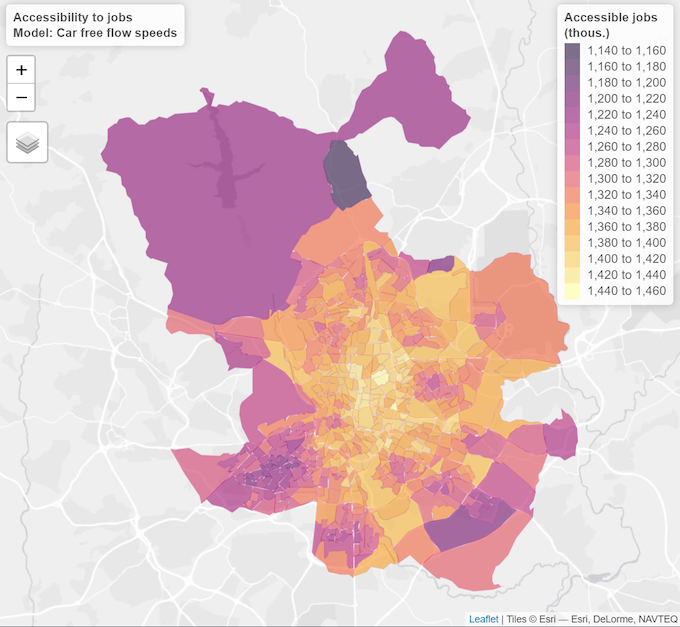
The map shows an total number of accessible jobs from a given location (transport zone), applying a typical commuting distance of inhabitants of Metropolitan area of Madrid (more details about used potential accessibility measure, can be found here).
Data used for this example can be downloaded from the github. The accessibility values were calculated for the MSCA CALCULUS project. The shapefiles of transport zones of Madrid can be downloaded from the open data portal of the Comunidad de Madrid (Delimitaciones Territoriales / Zonas de Transporte). In this map I use the zones dated for year 2013 limited to those located within the Municipality of Madrid (584 units).
Step 1. Load packages and get the data
library(readr)
library(dplyr)
library(tmap)
library(rgdal)
For the map we need a shapefile with transport zones of Madrid (Madrid_TAZ.shp) and csv file with accessibility values, both stored in the [Data] subfolder. The code below loads a shapefile (as SpatialPolygonsDataFrame) and merges it with the .csv. Additionally, the code recalculates the total number of accessible jobs (an original Ai_tmap.csv files contains results in thousands) which will be used in the popup.
Free.Flow <- merge(

      # read shapefile
      readOGR("Data/Madrid_TAZ.shp",
            layer = "Madrid_TAZ", GDAL1_integer64_policy = TRUE),

      # read csv file add a new column to be displayed in popup
      (read_csv("Data/Ai_tmap.csv") %>%
            mutate(K.FreeFlow = FreeFlow*1000) ),

      # matching columns
      by.x = "TAZ_Madr_1", by.y = "Or")
Step 2. Make a (t)map!
First, let’s set the tmap “view” mode:
tmap_mode("view")
The advantage of using tmap is that it shares a logic with ggplot. Thus, first we need to create a tmap object (tm_shape()) followed by a thematic layer (tm_polygons()), and then additional parameters (e.g. tm_layout()) should be specified. The subsequent elements we add using a +.
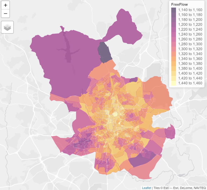
Let’s start with the first map using all default settings. We need to define the source of thematic layer (Free.Flow - a SpatialPolygonsDataFrame object) and a variable which defines a thematic layer (FreeFlow):
tm_shape(Free.Flow) +
    tm_polygons("FreeFlow")
Here it is! A first interactive map. In the top-left corner, we can turn off the visibility of our thematic layer and select one of the three default basemaps.
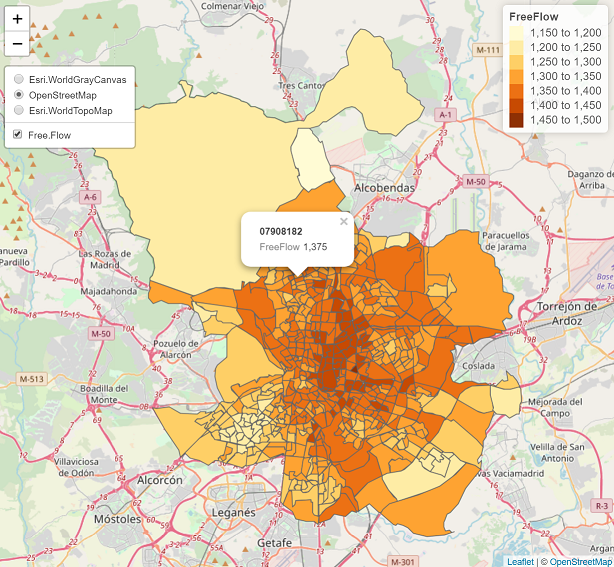
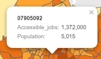
The popup shows us a value taken from the column used to create a thematic layer (FreeFlow) and it uses a first column to define area ID. We can change it now, using a popup.vars parameter of tm_polygons() function. The content of the popup is defined as: some.text = variable.name and a variable.name should be matched to the name of column of a thematic layer (as defined by tm_shape()). We use two columns: K.FreeFlow which contains a total number of available jobs, and POP2017 indicating a total number of population:
tm_shape(Free.Flow) +
    tm_polygons("FreeFlow",
                # popup definition
                popup.vars=c(
                    "Accessible_jobs: "="K.FreeFlow",
                    "Population: " = "POP2017")
                )
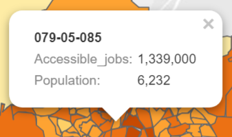
One remark: by default the popup uses a first column of our SpatialPolygonsDataFrame to display an area ID. We can use variables from another column by defining an id parameter:
tm_shape(Free.Flow) +
      tm_polygons("FreeFlow",

                    # popup definition
                    popup.vars=c(
                            "Accessible_jobs: "="K.FreeFlow",
                            "Population: " = "POP2017"),
                    id = "TAZ_Madrid"
        )
Now, let’s change the color palette and transparency of the thematic layer. I want to use the inferno palette - a viridis-based palette matched by {colorspace} team. I want to divide my data into as much as 16 classes. Additionally, I want to set the transparency of the thematic layer. In result, I need to define three parameters: palette, n (number of classes) and alpha (transparency):
        alpha = 0.6,
        n = 16,
        palette = hcl.colors(16, palette = "Inferno")
However, the darkest colors of the inferno palette are a bit too dark for me, so I want to exclude them. In order to do this, first I set more colors from the palette, and then filter out first two of them. Now, our code looks like this:
tm_shape(Free.Flow) +
        tm_polygons("FreeFlow",

                    # popup definition
                    popup.vars=c(
                            "Accessible_jobs: "="K.FreeFlow",
                            "Population: " = "POP2017"),
                    id = "TAZ_Madrid",

                    # transparency, number of classes and palette
                    alpha = 0.6,
                    n = 16,
                    palette = hcl.colors(18, palette = "Inferno")[3:18]
        )
The zones’ borders are too visible so we need to increase their transparency and change their color. I’ve tested several solutions taking an advantage of this on-line application and selected the one that fits the best:
tm_shape(Free.Flow) +
        tm_polygons("FreeFlow",

                    # popup definition
                    popup.vars=c(
                            "Accessible_jobs: "="K.FreeFlow",
                            "Population: " = "POP2017"),
                    id = "TAZ_Madrid",

                    # transparency, number of classes and palette
                    alpha = 0.6,
                    n = 16,
                    palette = hcl.colors(18, palette = "Inferno")[3:18],

                    # border definition: color and transparency
                    border.col = "#990099",
                    border.alpha = 0.1
        )
The map is almost ready. The last amendments: title of the legend and the map title. The previous is defined by the title parameter of tm_polygons() function, while the latter by a parameter of a separate function tm_layout():
tm_shape(Free.Flow) +
        tm_polygons("FreeFlow",

                    # popup definition
                    popup.vars=c(
                            "Accessible_jobs: "="K.FreeFlow",
                            "Population: " = "POP2017"),
                    id = "TAZ_Madrid",

                    # transparency, number of classes and palette
                    alpha = 0.6,
                    n = 16,
                    palette = hcl.colors(18, palette = "Inferno")[3:18],

                    # border definition: color and transparency
                    border.col = "#990099",
                    border.alpha = 0.1,

                    # title of the legend
                    title = "Accessible jobs<br>(thous.)"
        ) +

    # map title
    tm_layout(title = "Accessibility to jobs<br>Model: Car free flow speeds")
Note, that in both cases, a typical html tags (like <br>) can be used.
Step 3. Save and re-use the output
The map is ready!
Now, we only need to save it as a html widget. We can use a native tmap_save() function:
tmap_last() %>%
    tmap_save("Madrid_accessibility_map.html")
It can be then inserted to a web page:
<iframe src="/img/Madrid_accessibility_map.html" frameborder=0, height=400, width="100%", scrolling="no"></iframe>
All the code and the data can be downloaded from my github.
Session info:
R version 3.6.0 (2019-04-26)
Platform: x86_64-apple-darwin15.6.0 (64-bit)
Running under: macOS Mojave 10.14.5
Some useful links:
- tmap: get started!
- tmap in a nutshell
- The greate on-line course Using R for Data Journalism by Andrew Ba Tran
- The chapter in Geocomputation with R by Robin Lovelace, Jakub Nowosad and Jannes Muenchow