I have created my first (ever!) #rstats package. It is called {DepartureTime} and its purpose is to prepare a dataset with several departure times for temporally sensitive accessibility analysis.
What does {DepartureTime} do?
The package consists of one function which permits you to generate a series of departure times applying user-defined temporal resolution and one of four different sampling procedures:
- Systematic sampling method: departure times are selected using a regular interval defined by the frequency
- Simple Random sampling method: a specified number of departure times (defined by the frequency) is randomly selected from the time window
- Hybrid sampling method: departure times are randomly selected from given time intervals (resulted from applied temporal resolution)
- Constrained Random Walk Sampling sampling method: a first departure time is randomly selected from the subset of the length defined by the frequency and beginning of the time window; then, the next departure time is randomly selected from the subset limited by
\(Tn+f/2\)and\(Tn+f+f/2\).
An example of the result of sampling procedures for 20-minute temporal resolution and 1-hour-long time window (07:00-08:00) illustrates the following table:
| Sampling method | Departure times | Comments |
|---|---|---|
| Systematic | 07:00; 07:20, 7:40, 08:00 | regular interval of 20 minutes1 |
| Simple Random | 07:18; 07:51; 07:55 | 3 randomly selected departure times from the time window2 |
| Hybrid | 07:02; 07:23; 07:50 | One randomly selected departure time from each time interval period3 |
| Random Walk | 07:15; 07:36; 07:49 | on average there should be 20-minute interval between departure times4 |
1 as 20-minute interval fits to 60 minute time window it provides 4 departure times.
2 i.e. one per each 20 min. in 60-minute time window.
3 i.e. one from 07:00-07:19, one from 07:20-07:39 and one from 07:40-07:59.
4 due to the nature of the sampling procedure, the number of departure times might differ.
For details on sampling procedures, please consult Owen & Murphy (2018).
Why may you need {DepartureTime}?
Briefly: because, if you include temporal dimension to your accessibility analysis, the result depends on the applied departure time. In particular, in case of public transport, accessibility level in a given area might be highly affected by the fact whether you are “lucky” or not in terms of waiting times (for the first connection and/or in case of transfers) and, in result, these values might differ substantially just because you decided on a particular departure time. In order to limit this negative impact on analysis, you need to consider different departure times and than aggregate results in order to better reflect how does one experience level of accessibility.
Consider this graph presented by Owen & Levinson (2015):
*](/img/post/post_20200518/Owen_Levinson_2015.png) {width=400px}
{width=400px}
It shows how accessibility change over time for a selected census block. Depending on the selected departure time, you can get completely different accessibility level, even though the transport system nor the distribution of activities does not change.
Further, even if the level of availability does not change so drastically, you may still want to simulate different situation e.g. applying free flow, peak or out-of-peak speeds. The graph below, prepared for the Dutch case study, compares daily variation of job accessibility by car and by public transport (walk-and-ride and bike-and-ride models):
*](/img/post/post_20200518/Pritchard_et_al_2019.png)
Thus, regardless transport mode, you may need to repeat analysis without changing anything but departure time (even though, a required temporal resolution would change): in case of car accessibility you may need to generate origin-destination matrices couple of times during the day, while in case of public transport you should compute travel times even couple of times per hour (I you need more information on the consequences of applied temporal resolution on precision of accessibility analysis I can shamelessly suggest you the following paper: Stepniak, Pritchard, Geurs & Goliszek (2019)).
How can you take advantage of {DepartureTime}?
As described in the paper, you can select different approach how to tackle the issue of temporal resolution. Regardless which approach you select, you would need a table which contains all departure times in order to automatize calculations. I used it in ArcGIS Network Analyst (with Add GTFS to a Network Dataset tool), but as far as I know, {DepartureTime} may be also useful when working with OpenTripPlanner.
In ArcGIS you can easily prepare an arcpy code or just a ModelBuilder, which permits you to iterate by subsequent departure time. The simple ModelBuilder looks like this:
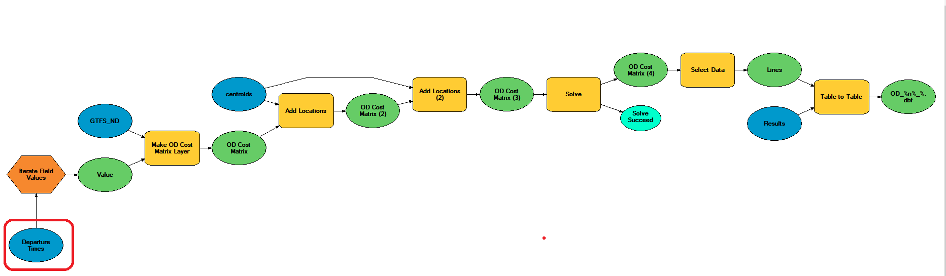*](/img/post/post_20200518/ModelBuilder.png)
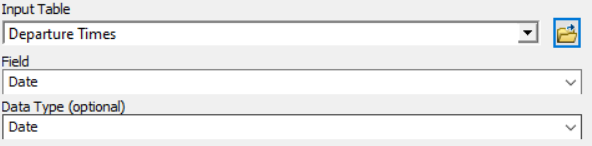
The .dbf file with the output from {DepartureTime} you need to locate in Departure Times (market with the red circle) and iterate it by Field Values (by Date field, setting Data type as Date)
In result of the above model, you obtain a set of origin-destination matrices, one for each of a departure time, exported to separate files (e.g. .dbf files). Then, they can be aggregated in order to obtain more realistic average travel time (or average accessibility), e.g. during the morning peak-hours or during the day (night etc.).
How does {DepartureTime} work?
The {DepartureTime} package can be installed in R directly from GitHub (if you don’t have {devtools} installed, you need to install it first):
# install.packages("devtools")
devtools::install_github("stmarcin/DepartureTime")
The function has the following syntax and default values:
DepartureTime <- function(method = "H",
                          dy = format(Sys.Date(), "%Y"),
                          dm = format(Sys.Date(), "%m"),
                          dd = format(Sys.Date(), "%d"),
                          tmin = 0, tmax = 24,
                          res = 5,
                          MMDD = TRUE,
                          ptw = FALSE)
Function variables:
method- sampling method; Options:RORRandom: Simple random sampling;SORSystematic: Systematic sampling;HORHybrid: Hybrid sampling;WORWalk: Constrained random walk sampling;
dy,dmanddd- date of the analysis (formats: YYYY, MM, DD); default: system date;tminandtmax- limits of the time window (format: HH); default: full day (00:00 - 24:00);res- temporal resolution; default: 5 minutesMMDD- date format of the output (TRUE / FALSE) default: TRUETRUE: MM/DD/YYYY;FALSE: DD/MM/YYYY;
ptw- print limits of subsetted time-windows; default: FALSE;
The DepartureTime() function creates a data frame with generated departure times, already formatted for ArcGIS:
| ColumnName | Description |
|---|---|
| ID | rowID (integer), starts with 0 |
| Date | Departure date & hour |
Example with selected user-defined parameters:
DepartureTime(method = "S",    # systematic sampling method
  dm = 5, dd = 15,             # user-defined date: 15th May, 2020 (current year)
  tmin = 7, tmax = 9,          # user-defined time window (07:00 - 09:00)
  res = 20)                    # user-defined temporal resolution (20 minutes)
| ID | Date |
|---|---|
| 0 | 05/15/2020 07:00 |
| 1 | 05/15/2020 07:20 |
| 2 | 05/15/2020 07:40 |
| 3 | 05/15/2020 08:00 |
| 4 | 05/15/2020 08:20 |
| 5 | 05/15/2020 08:40 |
| 6 | 05/15/2020 09:00 |
You can easily save {DepartureTime} output as .dbf file (you need to have {foreign} package installed):
library(DepartureTime)
library(foreign)
library(dplyr)

# generate departure times for 8-10am time window
# with 30-minute temporal resolution applying hybrid sampling model:
DepartureTime(tmin = 8, tmax = 10, res = 30) %>%

  #save output in OD_analysis subfolder as My_Departure_Times.dbf
  write.dbf("OD_analysis/My_Departure_Times.dbf")
Questions?
If you have any questions, feel free to contact me or fill an issue on github.
Further reading
Murphy, B., Owen, A., 2019. Temporal sampling and service frequency harmonics in transit accessibility evaluation Journal of Transport and Land Use 12, 893–913. https://doi.org/10.5198/jtlu.2019.1379
Owen, A., Levinson, D.M., 2015. Modeling the commute mode share of transit using continuous accessibility to jobs Transportation Research Part A: Policy and Practice 74, 110–122. https://doi.org/10.1016/j.tra.2015.02.002
Owen, A., Murphy, B., 2018. Temporal Sampling and Service Frequency Harmonics in Transit Accessibility Evaluation, in: Transportation Research Board 97th Annual Meeting. p. 10.
Pritchard, J.P., Stępniak, M., Geurs, K.T., 2019. Equity analysis of dynamic bike-and-ride accessibility in the Netherlands, in: Lucas, K., Martens, K., Ciommo, F. Di, Dupont-Kieffer, A. (Eds.), Measuring Transport Equity. Elsevier, pp. 73–83. https://doi.org/10.1016/B978-0-12-814818-1.00005-6
Stępniak, M., Pritchard, J.P., Geurs, K.T., Goliszek, S., 2019. The impact of temporal resolution on public transport accessibility measurement: Review and case study in Poland Journal of Transport Geography 75, 8–24. https://doi.org/10.1016/j.jtrangeo.2019.01.007